회귀(regression) 분석 활용 및 예시

import pandas as pd

dataIn = './../dataIn/'

pd.set_option('display.max_columns', None)

df = pd.read_csv(dataIn + 'auto-mpg.csv', header=None)
df.columns = ['mpg', 'cylinders', 'displacement', 'housepover', 'weight', 'accelerations', 'model_year', 'origin', 'name']
print('\n데이터 살펴 보기')
print(df.head())

print('\n데이터 자료형 확인')
print(df.info())

 

 

 

print('\n데이터 통계 정보 요약')
print(df.describe())

 

 

print('\n컬럼별 누락 데이터 확인')
print(df.isnull().sum())

import seaborn as sns
import matplotlib.pyplot as plt

plt.rc('font', family='Malgun Gothic')
# 음수 부호 경고 메시지 없애기
plt.rcParams['axes.unicode_minus'] = False

dataOut = './../dataOut/'

sns.pairplot(df)

filename = dataOut + 'pairplot.png'
plt.savefig(filename)
print(f'{filename} 파일 저장')

 

print('\n상관 계수')
corr = df.corr(numeric_only=True)
print(corr)

 

 

 

import numpy as np

plt.figure(figsize=(10,8))
mask = np.triu(np.ones_like(corr, dtype=bool))

plt.rc('font', family='Malgun Gothic')

# 음수 부호 경고 메시지 없애기
plt.rcParams['axes.unicode_minus'] = False
sns.heatmap(corr, mask=mask, cmap='coolwarm', annot=True, fmt='.2f', cbar=True)
plt.title('변수들간 상관 계수', size=15)
plt.savefig(dataOut + 'corr_heatmap.png')

 

 

print('\nhorsepower 컬럼의 고유한 값 확인')
print(df['horsepower'].unique())

# 마력이 '?'인 항목 개수 파악
print('\n빈도수 역순으로 조회')
print(df['horsepower'].value_counts())

 

 

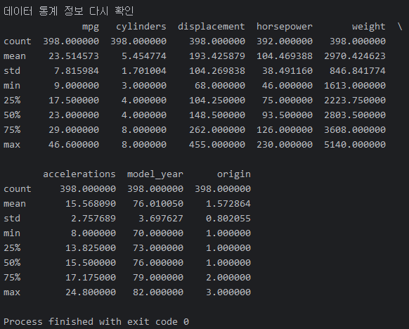
df['horsepower'] = df['horsepower'].replace('?', np.nan)
df['horsepower'] = df['horsepower'].astype('float')

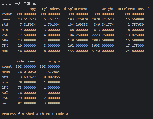
print('\n데이터 통계 정보 다시 확인')
print(df.describe())

 

 

print('\n결측치 제거전 : ' +  str(df['horsepower'].isnull().sum()))
df_nan = df.dropna(subset=['horsepower'], axis=0)
print('\n결측치 제거후 : ' +  str(df_nan['horsepower'].isnull().sum()))

 

 

# 결측치들을 비결측치들의 평균 값으로 대체하도록 합니다.
print('\n결측치 제거전 : ' +  str(df['horsepower'].isnull().sum()))
df['horsepower'] = df['horsepower'].fillna(df['horsepower'].mean())
print('\n결측치 제거후 : ' +  str(df['horsepower'].isnull().sum()))

 

 

print('\n분석에 필요한 열(feature_특성)만 추출하기')
print('연비, 실린더, 마력(출력), 중량')
ndf = df[['mpg','cylinders','horsepower','weight']]

print('다중 회귀 분석을 위하여 복사본을 생성합니다.')
# xxx = ndf # 참조 복사
multidf = ndf.copy() # 참조 복사가 아닌 값 복사를 수행합니다.

 

 

 

import numpy as np

plt.figure(figsize=(10,8))
mask = np.triu(np.ones_like(corr, dtype=bool))

plt.rc('font', family='Malgun Gothic')

# 음수 부호 경고 메시지 없애기
plt.rcParams['axes.unicode_minus'] = False
sns.heatmap(corr, mask=mask, cmap='coolwarm', annot=True, fmt='.2f', cbar=True)
plt.title('변수들간 상관 계수', size=15)
plt.savefig(dataOut + 'corr_heatmap_new.png')

 

 

print('`연비`와 `무게`의 산점도 그래프')
plt.figure(figsize=(10,8))
sns.scatterplot(data=ndf, x='weight', y='mpg')
plt.title('`연비`와 `무게`의 산점도 그래프', size=15)
filename = 'scatterplot.png'
plt.savefig(dataOut + filename)
print(f'{filename} 파일 생성됨')

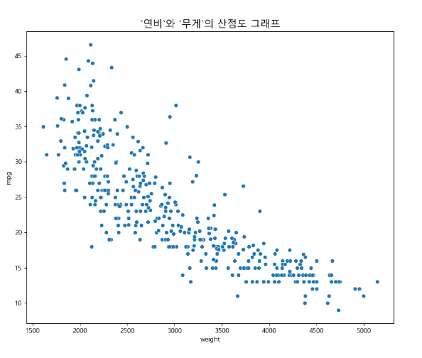
# 독립 변수를 사용하여 종속 변수에 대한 단순 회귀 분석 테스트
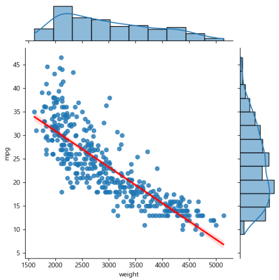
# 회귀선 표시
plt.figure(figsize=(10,8))
# kind='reg' : 회귀선(regression Line) 표시
sns.jointplot(data=ndf, x='weight', y='mpg', kind='reg', line_kws={'color':'red'})
filename = 'jointplot.png'
plt.savefig(dataOut + filename)
print(f'{filename} 파일 생성됨')

 

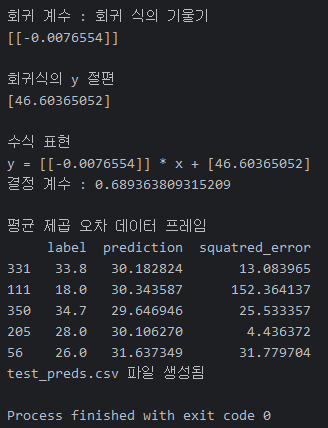
# prediction은 머신 러닝이 학습한 모델을 이용하여 예측해준 정보
prediction = model.predict(x_test)

# 오차(잔차) 계산
test_preds = pd.DataFrame()
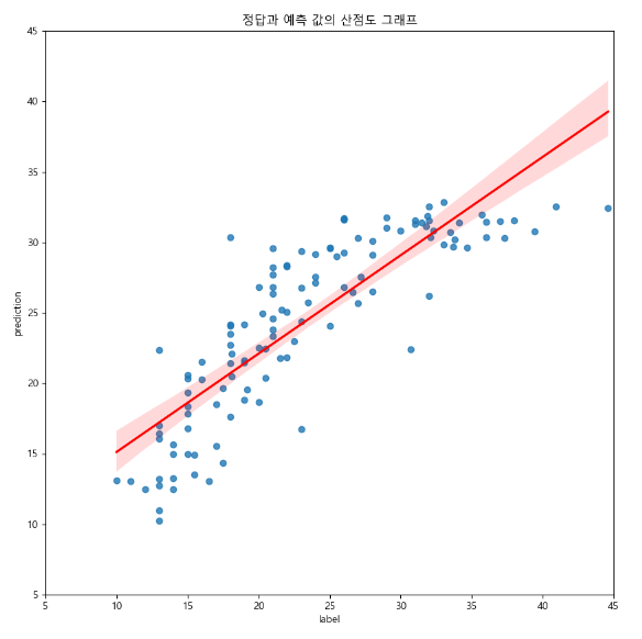
test_preds['label'] = y_test # 실제 정답 데이터를 의미하는 label
test_preds['prediction'] = prediction # 학습한 모델이 예측해준 정보
# (실제정답 - 예측값)의 제곱
test_preds['squatred_error'] = (test_preds['label'] - test_preds['prediction']) ** 2

print('\n평균 제곱 오차 데이터 프레임')
print(test_preds.head())

filename = 'test_preds.csv'
test_preds.to_csv(dataOut + filename, index=False)
print(f'{filename} 파일 생성됨')

# 평균 제곱 오차(mean squared error)
mse = test_preds['squatred_error'].mean()
print(mse)

 

 

print('산점도와 회귀선')
plt.figure(figsize=(10, 10))

sns.regplot(x='label', y='prediction', data=test_preds, line_kws={'color':'red'})
plt.title('정답과 예측 값의 산점도 그래프')
plt.xlim([5, 45])
plt.ylim([5, 45])
filename = 'regplot.png'
plt.savefig(dataOut +  filename)
print(filename + '파일이 저장되었습니다.')