클래스 분류와 의사 결정 트리의 활용 예시

Jun's Blog

클래스 분류와 의사 결정 트리의 활용 예시 본문

카테고리 없음

클래스 분류와 의사 결정 트리의 활용 예시

luckydadit 2025. 3. 21. 14:56

의사 결정 트리는 데이터를 분류하거나 예측하기 위한 트리 구조의 모델이에요. 이 모델은 주어진 데이터를 여러 특성(feature)을 기준으로 분할하면서 최종적인 예측을 하게 됩니다.

엔트로피는 정보 이론에서 나온 개념으로, 주어진 데이터의 불확실성이나 혼잡도를 측정하는 지표입니다.
의사 결정 트리에서는 데이터를 얼마나 잘 분할할 수 있는지 평가할 때 사용됩니다.
엔트로피가 높을수록 데이터의 불확실성이 크고, 낮을수록 데이터의 불확실성이 적다는 의미입니다.

from collections import Counter

ball_list = ['red', 'blue', 'red', 'blue', 'red', 'blue', 'red']

counter = Counter(ball_list)
print(counter)

total_cnt = len(ball_list)

# 각 항목의 비율 계산
ratios = {key:value/total_cnt for key, value in counter.items()}
print(ratios)

# 각 항목의 비율 계산
ratios = {key:value/total_cnt for key, value in counter.items()}
print(ratios)

# 각 항목의 결과 출력
for color, ratio in ratios.items():
    print(f'{color}: {ratio:.5f}')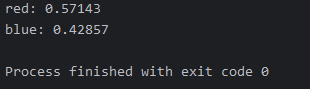

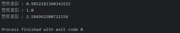
def shannon_entropy(probabilities):
    probabilities = np.array(probabilities)

    entropy = - np.sum(probabilities * np.log2(probabilities))
    print(f'엔트로피 : {entropy}')
# end def shannon_entropy(probabilities)

probabilities = [value for value in ratios.values()]
shannon_entropy(probabilities)

# 동전 던지기
probabilities = [0.5, 0.5]
shannon_entropy(probabilities)

# 주사위 던지기
probabilities = [1/6, 1/6, 1/6, 1/6, 1/6, 1/6]
shannon_entropy(probabilities)

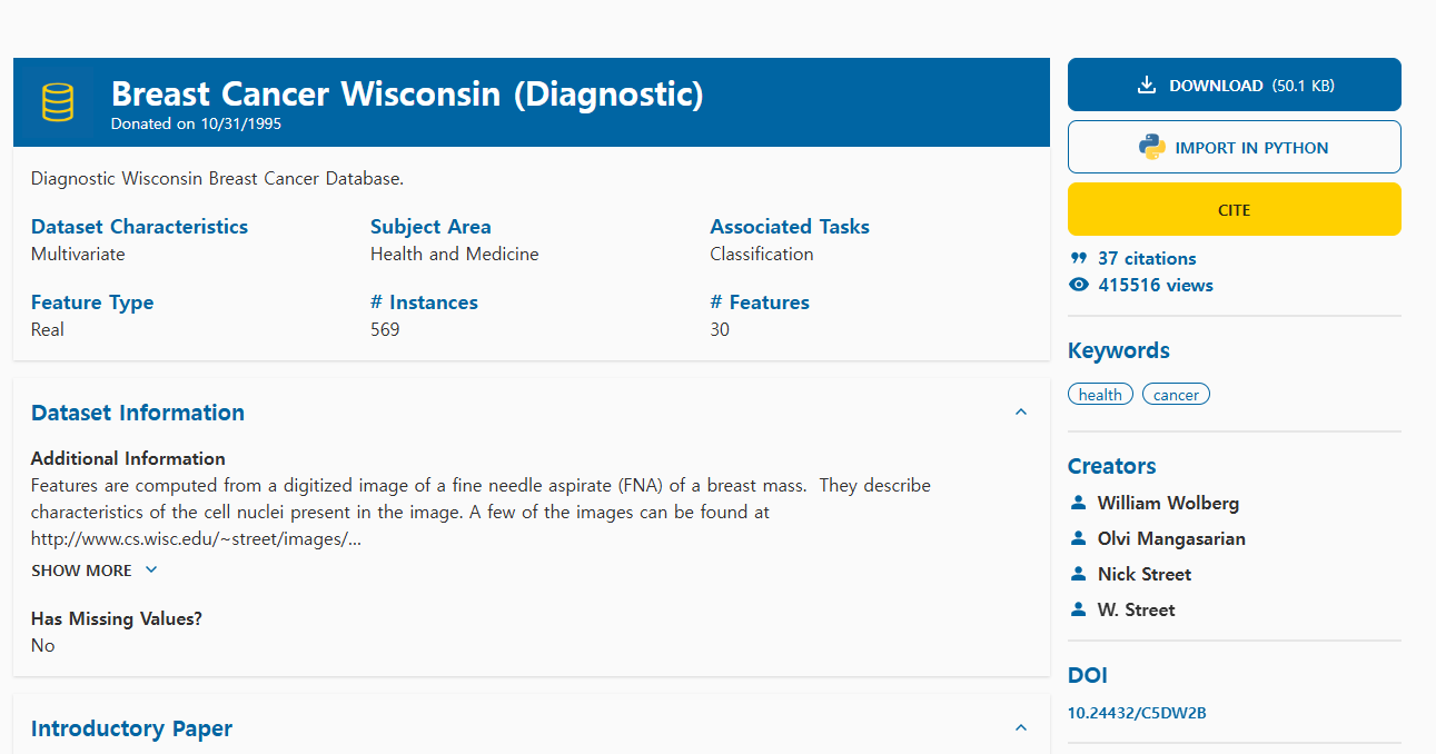
https://archive.ics.uci.edu/dataset/17/breast+cancer+wisconsin+diagnostic

UCI Machine Learning Repository

This dataset is licensed under a Creative Commons Attribution 4.0 International (CC BY 4.0) license. This allows for the sharing and adaptation of the datasets for any purpose, provided that the appropriate credit is given.

archive.ics.uci.edu

import numpy as np
import pandas as pd
import seaborn as sns
import matplotlib.pyplot as plt
from IPython.core.pylabtools import figsize

dataIn, dataOut = './../dataIn/', './../dataOut/'

plt.rc('font', family='Malgun Gothic')
plt.rcParams['axes.unicode_minus'] = False

uci_path = dataIn + 'breast-cancer-wisconsin.data.txt'
# index_col='id' : 파일을 읽어 들이면서 id 컬럼은 색인으로 옮겨 주세요.
df = pd.read_csv(uci_path, index_col='id')

print(f'데이터 셋의 크기 : {df.shape}')

print('\n 데이터 살펴보기')
print(df.head())

print('\n 데이터 자료형 확인')
print(df.info())

print('\n 데이터 통계 요약 정보 확인')
print(df.describe(include='all'))

print('\n 누락된 데이터 확인')
print(df.isnull().sum())

print('\n 중복된 데이터 개수')
print(df.duplicated().sum())

print('\n 종속 변수 확인')
print(df['class'].value_counts())

범주형 데이터 일경우에만 unique, top, freq가 존재함. 아니면 연속형 데이터를 의미함. unique : 카테고리 수, top : 가장 많이 나온 값, freq : top의 값이 중복된 횟수

print('\n 종속 변수 확인')
print(df['class'].value_counts())

# 종속 변수를 이진 변수로 변환
df['class'] = df['class'].map({2:0, 4:1})

print('\n 종속 변수 확인(비율)')
print(df['class'].value_counts(normalize=True))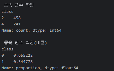

# 히스토 그램 시각화
df.hist(figsize=(15, 12))
filename = dataOut + 'breast_image01.png'
plt.title('')
plt.savefig(filename)
print(f'{filename} 파일이 저장되었습니다.')

print(df['bare_nuclei'].unique())

print(df['bare_nuclei'].value_counts())

df['bare_nuclei'] = df['bare_nuclei'].replace('?', np.nan)
df = df.dropna(subset=['bare_nuclei'], axis=0)
df['bare_nuclei'] = df['bare_nuclei'].astype('int')

print(df['bare_nuclei'].unique())

print(df['bare_nuclei'].value_counts())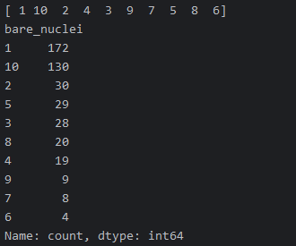

# 독립 변수와 종속 변수 분리
independent_variable = ['clump', 'cell_size', 'cell_shape', 'adhesion', 'epithlial', 'bare_nuclei', 'chromatin', 'normal_nucleoli']

x = df[independent_variable] # 독립 변수
y = df['class'] # 종속 변수

# 데이터 정규화
scalar = StandardScaler()
scalar.fit(x)
x = scalar.transform(x)

x_train, x_test, y_train, y_test = \
    train_test_split(x, y, test_size=0.3, random_state=10)

model = DecisionTreeClassifier(criterion='entropy', max_depth=5)

model.fit(x_train, y_train)

prediction = model.predict(x_test)

# 모형 성능 평가 - Confusion Matrix 계산
tree_matrix = confusion_matrix(y_test, prediction)
print('tree_matrix')
print(tree_matrix)

# Confusion Matrix 시각화
plt.figure(figsize=(8, 6))
sns.heatmap(tree_matrix, annot=True, fmt='d', cmap='Greens',
            xticklabels=['Positive', 'Negative'],
            yticklabels=['Positive', 'Negative'])

plt.title('Confusion Matrix')
plt.ylabel('Actual label')
plt.xlabel('Predicted label')
plt.savefig(dataOut + 'confusion_matrix.png')

# 모형 성능 평가 - 평가 지표 계산
tree_report = classification_report(y_test, prediction)
print(tree_report)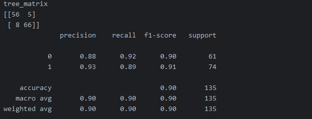

features = pd.DataFrame(model.feature_importances_, index=independent_variable, columns=['Importance'])

# 값을 기반으로 역순으로 정렬해 주세요.
features = features.sort_values(by='Importance', ascending=False)
print(features)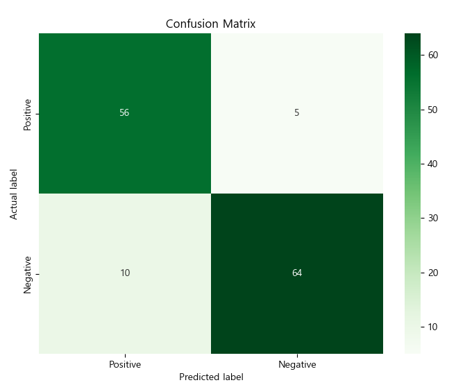

# 값을 기반으로 역순으로 정렬해 주세요.
features = features.sort_values(by='Importance', ascending=False)
print(features)

max_index = features['Importance'].idxmax()
print(f'Importance 컬럼에서 가장 중요한 결정 요소 : {max_index}')
print(f'해당 색인의 값 : {features.loc[max_index, "Importance"]}')

plt.figure(figsize=(10, 6))

sns.barplot(x=features.Importance, y=features.index, hue=features.index, palette='viridis')

print('특성 중요도에 대한 시각화')
filename = dataOut + 'barplot.png'
plt.title('특성 중요도 시각화')
plt.xlabel('Importance')
plt.ylabel('Feature')
plt.savefig(filename)
print(f'{filename} 파일이 저장되었습니다.')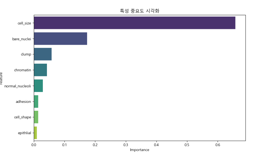

print('의사 결정 트리 시각화')
plt.figure(figsize=(20, 10))
plot_tree(model,
           feature_names=independent_variable,
           class_names=['Benign','Malignant'], # 양성, 악성
           filled=True,
           rounded=True,
           fontsize=12)
filename = dataOut + 'decision_plot_tree.png'
plt.title('Decision Tree Visualization')
plt.savefig(filename)
print(f'{filename} 파일 저장되었습니다.')

print(f'트리의 최대 깊이 : {model.get_depth()}')
print(f'리프 노드 갯수 : {model.get_n_leaves()}')

# HyperParameter는 모델이 학습하기 전에 개발자가 설정해야 하는 어떠한 값을 말합니다.
print(f'하이퍼 파라미터 정보 : \n', model.get_params())

print(f'특성 중요도 출력: \n, {model.feature_importances_}')

tree_rules = export_text(model, feature_names=independent_variable)
print(tree_rules)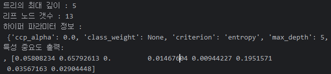

<print(tree_rules) 결과>

Jun's Blog

클래스 분류와 의사 결정 트리의 활용 예시 본문

클래스 분류와 의사 결정 트리의 활용 예시

티스토리툴바