클래스 분류의 정의와 SVM의 활용 예시 - (1)

클래스 분류(Classification)는 주어진 입력 데이터를 여러 카테고리(클래스) 중 하나로 분류하는 것을
의미합니다.


SVM(Support Vector Machine)은 이러한 클래스 분류 문제를 해결하는 데 사용되는 강력한 알고리즘 중 하나입니다. SVM은 데이터를 최적으로 분리하는 경계를 찾는 방법입니다.

 

 

1. seaborn 라이브러리에 제공되는 타이타닉(titanic)을 활용하여 SVM 실습 해보기

import seaborn as sns

df = sns.load_dataset('titanic')
print(type(df))
print(df.columns)

print(df['survived'].value_counts())

print('중복되는 행의 개수 : ' +  str(sum(df.duplicated())))

# 중복된 데이터 삭제
print('before drop duplicated : ' +  str(len(df)))
df = df.drop_duplicates()
print('after drop duplicated : ' +  str(len(df)))

print('df.info()')
print(df.info())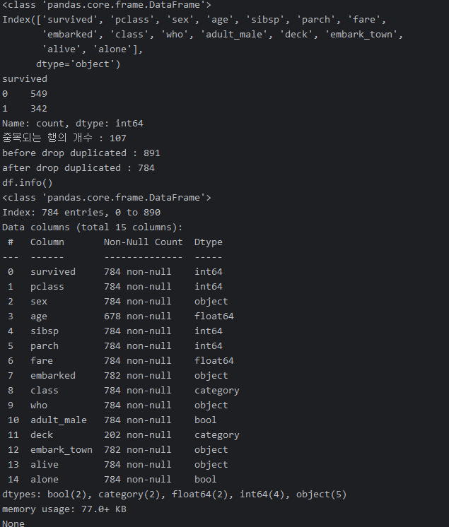

 

print(df[['embarked', 'embark_town']].head(10))

# 결측치가 많은 'deck'와 의미가 중복되는 'embark_town'는 삭제
rdf = df.drop(['deck', 'embark_town'], axis=1)

# how='any' 옵션은 해당 행또는 열에 결측치가 1개 이상이면 제거합니다.
rdf = rdf.dropna(subset=['age'], how='any', axis=0)

print(df['embarked'].unique())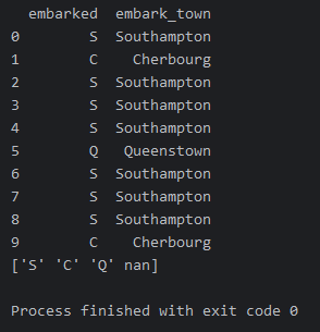

 

# 승선 위치 중 결측치(범주형 데이터일 경우)는 가장 많이 승선한 도시의 값으로 치환합니다.
# ['S' 'C' 'Q' nan]
print(df['embarked'].unique())
print(df['embarked'].value_counts())

most_frequency = rdf['embarked'].mode()[0]
print(f'most_frequencty={most_frequency}')
rdf['embarked'] = rdf['embarked'].fillna((most_frequency))

 

# 분석에 사용할 열(특성)만 선택
ndf = rdf[['survived', 'pclass', 'sex', 'age', 'sibsp', 'parch', 'embarked']]

print(ndf.columns)
print(ndf.head(5))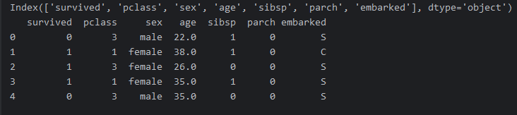

 

# 범주형 데이터를 모델이 인식할 수 있도록 숫자형으로 변환
import pandas as pd

trans_sex = pd.get_dummies(data=ndf['sex'], dtype=int)
trans_embarked = pd.get_dummies(data=ndf['embarked'], prefix='town', dtype=int)
ndf = pd.concat([ndf, trans_sex, trans_embarked], axis=1)

pd.set_option('display.max_columns', None)

ndf = ndf.drop(['sex', 'embarked'], axis=1)
print(ndf.head())
print(ndf.columns)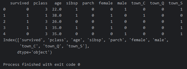

 

SVM에서 StandardScaler(표준화 스케일러)를 사용하는 이유는
모델 성능 향상과 알고리즘의 정확한 작동을 위해서입니다.
SVM은 거리 기반 모델이기 때문에 입력 데이터의 스케일에 민감합니다.
이를 해결하기 위해 데이터 전처리 단계에서 StandardScaler를 사용해 데이터를 표준화하는 것이 매우 중요합니다.

 

# 독립 변수와 종속 변수 분리
x = ndf[['pclass', 'age', 'sibsp', 'parch', 'female', 'male',
       'town_C', 'town_Q', 'town_S']]
y = ndf['survived']

print('before normalization')
print(x[:5])

scaler = StandardScaler()
x = scaler.fit(x).transform(x)

print('after normalization')
print(x[:5])

 

x_train, x_test, y_train, y_test = \
    train_test_split(x, y, test_size=0.3, random_state=10)

# 모델 생성
model = SVC(kernel='rbf', probability=True)

model.fit(x_train, y_train)

prediction = model.predict(x_test)

print('예측 값')
print(prediction[0:10])

# 판다스 시리즈 y_test를 넘파이 배열로 변경하기 위하여 values 속성을 사용합니다.
print('실제 정답 데이터')
print(y_test.values[0:10])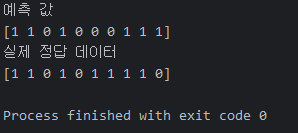

 

# 분류 모델 성능 평가
# confusion_matrix(실제정답데이터, 예측한값)
svm_matrix = confusion_matrix(y_test, prediction)
confusion_matrix(y_test, prediction)
print(svm_matrix)

 

 

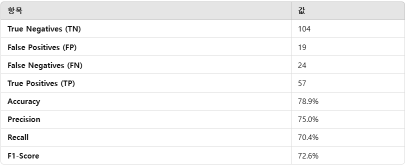
• True Negatives (TN): 104
  • 실제: 0, 예측: 0인 경우입니다.
  • 즉, 실제로 클래스 0에 속하는 샘플이 클래스 0으로 올바르게 예측된 수입니다.
• False Positives (FP): 19
  • 실제: 0, 예측: 1인 경우입니다.
  • 즉, 실제로 클래스 0에 속하는 샘플이 클래스 1로 잘못 예측된 수입니다.
• False Negatives (FN): 24
  • 실제: 1, 예측: 0인 경우입니다.
  • 즉, 실제로 클래스 1에 속하는 샘플이 클래스 0으로 잘못 예측된 수입니다.
• True Positives (TP): 57
  • 실제: 1, 예측: 1인 경우입니다.
  • 즉, 실제로 클래스 1에 속하는 샘플이 클래스 1으로 올바르게 예측된 수입니다.

 

 

# 기본 라이브러리 불러오기
import matplotlib.pyplot as plt
plt.rc('font', family='Malgun Gothic')
plt.rcParams['axes.unicode_minus'] = False

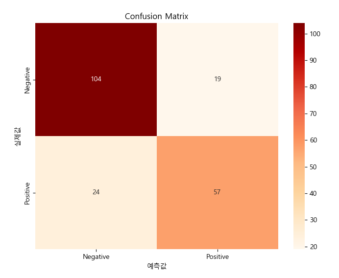
# Confusion Matrix 시각화
plt.figure(figsize=(8, 6))
sns.heatmap(svm_matrix, annot=True, fmt='d', cmap='OrRd',
            xticklabels=['Negative', 'Positive'],
            yticklabels=['Negative', 'Positive'])

plt.title('Confusion Matrix')
plt.ylabel('실제값')
plt.xlabel('예측값')

dataOut = './../dataOut/'

filename = dataOut + 'svm_titanic_image_01.png'
plt.savefig(filename)
print(filename + ' 파일이 저장되었습니다.')

 

svm_report = classification_report(y_test, prediction)
print(svm_report)

prediction_probability = model.predict_proba(x_test)
print(prediction_probability[0:3])

# 생존일 확률 정보만 따로 추출합니다.
alive_probability = prediction_probability[:, 1]

# ROC 커브 만들기
fpr, tpr, thresholds = roc_curve(y_test, alive_probability)

roc_auc = auc(fpr, tpr)

plt.rc('font', family='Malgun Gothic')
plt.rcParams['axes.unicode_minus'] = False

# Confusion Matrix 시각화
plt.figure(figsize=(8, 8))

plt.plot(fpr, tpr, color='darkorange', lw=2, label=f'ROC curve (AUC = {roc_auc:.2f}')
plt.plot([0,1], [1,0], color='navy', lw=2, linestyle='--')
plt.xlim([0.0, 1.0])
plt.ylim([0.0, 1.0])
plt.title('ROC 커브')
plt.ylabel('True Positive Rate')
plt.xlabel('False Positive Rate')
# plt.legend(loc='lower right')

dataOut = './../dataOut/'

filename = dataOut + 'svm_titanic_roc_curve.png'
plt.savefig(filename)
print(filename + ' 파일이 저장되었습니다.')